Building a Hybrid Data Warehouse Model
Developer: Business Intelligence
by James Madison
As suggested by this reference implementation, in some cases blending the relational and dimensional models may be the right approach to data warehouse design.
Published April 2007
Relational and dimensional modeling are often used separately, but they can be successfully incorporated into a single design when needed. Doing so starts with a normalized relational model and then adds dimensional constructs, primarily at the physical level. The result is a single model that can provide the strengths of its parent models fairly well: it represents entities and relationships with the precision of the traditional relational model, and it processes dimensionally filtered, fact-aggregated queries with speed approaching that of the traditional dimensional model.
DOWNLOAD
Real-world experience was the motivation for this analysis: on three separate data warehousing projects where I worked as programmer, architect, and manager, respectively, I found a consistent pattern of data/database behavior that lent itself far more to a hybrid combination of dimensional and relational modeling than to either one alone.
This article discusses the hybrid design and provides a fully functional reference implementation. The system runs on Oracle Database 10g. It contains all code needed to build the database schemas, generate sample data, load it into the schemas, build the indexes and materialized views, run the sample queries, capture the runtimes, and provide statistics on the runtimes.
The hybrid model is not a one-size-fits-all solution. Many projects are best served by either using only one of the traditional models or using both models separately with a feed between them. But if the objective is to create a single database that can both store data in its properly normalized form and run aggregation queries with good performance, the hybrid model is a design pattern to consider.
Sample Business Domain
The sample business domain is in the insurance industry and uses the following entities:
| Entity | Description |
|---|---|
| ACCOUNT | Information about a customer and its activities with the insurance company |
| POLICY | An insurance contract representing a specific agreement with the customer |
| VEHICLE | A vehicle belonging to the customer and covered by a policy |
| COVERAGE | The kinds of losses that are covered for a vehicle on this policy |
| PREMIUM | A monthly payment from the customer for coverage on vehicles in this policy |
The sample business questions used to analyze the performance of the system have some parallel with reality but also cover extremes of behavior: scanning the fact table for many rows, retrieving a tiny percentage of fact rows, restricting to only the top table, restricting to every table, restricting to only the lower tables, and so on. They are the kinds of questions business users ask of dimensional models, not the kinds of questions that are typically asked of relational models. The relational model questions are not addressed, because it is assumed that the relational model will outperform the dimensional model for questions of a relational nature, such as "Show me all the vehicles on this policy." The questions used in this analysis are the following:
| ID# | Business Questions of a Dimensional Nature |
|---|---|
| 1 | What was the total premium collected by year as far back as we can go? |
| 2 | What was the premium collected in the New England states in 2002? |
| 3 | How much premium did we get for medium catastrophe risks in Connecticut as far back as we can go? |
| 4 | How much premium did we get for time-managed plan types in California in 2001? |
| 5 | How many passenger cars had collision coverage in November 2003? |
| 6 | What was the premium for red vehicles in Vermont with primary usage that had a $1,000 deductible? Break the numbers down per person and by accident limits. |
| 7 | What was the premium for coverages with a $1,000 deductible, a $100,000 per-person limit, and an $800,000 accident limit in 2000? |
| 8 | What was the monthly premium in 1999 for red cars with 750cc engines? |
Models
The three models are presented in Figures 1, 2, and 3. The hybrid model is based on the relational model, with two changes that derive from dimensional modeling practices: (1) Create a relationship from the PREMIUM table to each table in the upper portion of the hierarchy, and (2) Add the time dimension.
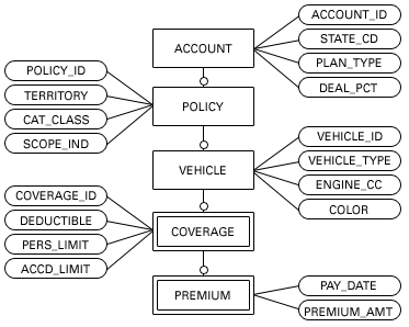
Figure 1. Relational model

Figure 2. Dimensional model

Figure 3. Hybrid model
Implementation
Largely standard techniques were used to convert the models into their physical implementation in database schemas. The relational schema was created with normalized modeling techniques, and the dimensional schema was done according to Ralph Kimball's work. Creating the hybrid meant copying the relational schema and then layering the dimensional constructs on top of it. (The " File Descriptions" sidebar lists the most important files in the implementation--which includes those files with DDL, the system validation, the queries, and the automated analysis used to generate the sample code.)
Because only three nonkey attributes are used, a SIZING attribute is added to each table, with a type of CHAR(100) to make the row size more realistic.
Certain database parameters must be set so that star joins will occur and materialized views will be used. The important parameters are shown here:
NAME                           VALUE
------------------------------ --------------------
compatible                     10.2.0.1.0
optimizer_features_enable      10.2.0.1
optimizer_mode                 first_rows
pga_aggregate_target           83886080
query_rewrite_enabled          true
query_rewrite_integrity        stale_tolerated
sga_target                     167772160
star_transformation_enabled    true
Verifying that a star join is occurring is done with EXPLAIN PLAN, as detailed in Oracle documentation.
All three schemas were loaded with the same data. The best evidence of consistent data loading is that all three schemas produce the same answers for the sample queries.
The volume of data used for the analysis is shown below.
OWNER  TABLE_NAME     NUM_ROWS AVG_ROW_LEN LAST_ANALYZED
------ ------------ ---------- ----------- -------------------
DIM    ACCOUNT_DIM        2000         128 2006-01-14:19-51-56
       COVERAGE_DIM        900          17 2006-01-14:19-51-57
       POLICY_DIM         6000         128 2006-01-14:19-51-58
       PREMIUM_FACT    1371183          23 2006-01-14:19-52-14
       TIME_DIM           3600          21 2006-01-14:19-52-39
       VEHICLE_DIM       24000         130 2006-01-14:19-52-39
HYB    ACCOUNT            2000         128 2006-01-14:19-53-42
       COVERAGE         144000          28 2006-01-14:19-53-47
       POLICY             6000         142 2006-01-14:19-53-53
       PREMIUM         1373463          49 2006-01-14:19-54-41
       TIME_DIM           3600          21 2006-01-14:19-55-08
       VEHICLE           24000         144 2006-01-14:19-55-10
REL    ACCOUNT            2000         124 2006-01-14:19-39-22
       COVERAGE         144288          27 2006-01-14:19-39-30
       POLICY             6000         138 2006-01-14:19-39-31
       PREMIUM         1389963          29 2006-01-14:19-40-08
       VEHICLE           24000         139 2006-01-14:19-40-13
The goal was to provide a sufficiently large volume to prevent the optimizer from taking shortcuts, such as reading entire tables instead of using indexes and other such optimization techniques that would undermine the analysis. According to Oracle Database Data Warehousing Guide 10 g Release 2 (10.2), Schema Modeling Techniques, a star transformation might not occur if the optimizer finds "tables that are too small for the transformation to be worthwhile."
A fairly arbitrary goal of the implementation was to have at least 1 million rows in the fact table. Given that all dimensional and hybrid query plans generated by QUERIES.SQL meet the criteria of star joins, the data volume used appears to be sufficient for the current analysis.
The number of COVERAGE_DIM rows is smaller in the dimensional schema than in the DIMENSION tables of the other two schemas because of the way a weak entity has to be represented in the dimensional schema.
Here is the amount of space consumed by the various schemas:
OWNER           TOTAL_SIZE
--------------- ----------------
DIM                  129,499,136
HYB                  244,056,064
REL                  130,023,424
Because the hybrid schema is a combination of the relational and the dimensional, it follows that it should be roughly the size of both, minus any common elements, and the numbers bear this out.
Running the System
Each of the queries was run 21 times, and the median runtime was used as the representative value, as shown below.
EVENT WINNER_TIME          RNR_UP_TIME          LOSER_TIME
----- -------------------- -------------------- --------------------
1.    DIM = 00:00:06.049   REL = 00:00:09.023   HYB = 00:00:09.644
2.    DIM = 00:00:04.186   HYB = 00:00:07.961   REL = 00:00:08.092
3.    DIM = 00:00:03.415   HYB = 00:00:04.938   REL = 00:00:05.428
4.    DIM = 00:00:00.140   HYB = 00:00:00.190   REL = 00:00:06.990
5.    HYB = 00:00:00.131   DIM = 00:00:00.651   REL = 00:00:05.418
6.    DIM = 00:00:00.530   HYB = 00:00:01.392   REL = 00:00:05.478
7.    DIM = 00:00:00.520   HYB = 00:00:01.572   REL = 00:00:07.9718.


DIM = 00:00:00.461   HYB = 00:00:00.731   REL = 00:00:01.882
Converting to a percentage scale, to make the values relative rather than absolute, and forcing the fastest schema to 100 percent by definition produces these percentages:
EVENT WINNER_OFFSET        RNR_UP_OFFSET        LOSER_OFFSET
----- -------------------- -------------------- --------------------
1.    DIM =    100%        REL =    149%        HYB =    159%
2.    DIM =    100%        HYB =    190%        REL =    193%
3.    DIM =    100%        HYB =    145%        REL =    159%
4.    DIM =    100%        HYB =    136%        REL =   4993%
5.    HYB =    100%        DIM =    497%        REL =   4136%
6.    DIM =    100%        HYB =    263%        REL =   1034%
7.    DIM =    100%        HYB =    302%        REL =   1533%
8.    DIM =    100%        HYB =    159%        REL =    408%
Comparing Relational and Dimensional
Showing that the dimensional schema outperforms the relational schema when running dimensional queries functions as the control of the experiment and provides the baseline from which to consider the hybrid schema's performance. As you can see below, the dimensional schema consistently outperforms the relational schema, as expected.
EVENT WINNER_OFFSET        RNR_UP_OFFSET        LOSER_OFFSET
----- -------------------- -------------------- --------------------
1.    DIM =    100%        REL =    149%
2.    DIM =    100%                             REL =    193%
3.    DIM =    100%                             REL =    159%
4.    DIM =    100%                             REL =   4993%
5.                         DIM =    497%        REL =   4136%
6.    DIM =    100%                             REL =   1034%
7.    DIM =    100%                             REL =   1533%
8.    DIM =    100%                             REL =    408%
In the case of Query #4, the difference is nearly 50-fold! Query #4 is the most extreme case in which the only (nontime) restriction is on attributes of the topmost table. In the relational schema, this means that all the tables down the hierarchy must be joined to get to the numerical information—an expensive operation. In the dimensional schema, the join is a direct connection from one dimension right into the fact table—an efficient operation.
Hybrid vs. Dimensional
Whether the hybrid schema performs as well as the dimensional is the core question in this analysis. As you can see below, the hybrid schema works reasonably well, but the hybrid approach is not as fast as a purely dimensional one.
EVENT WINNER_OFFSET        RNR_UP_OFFSET        LOSER_OFFSET
----- -------------------- -------------------- --------------------
1.    DIM =    100%                             HYB =    159%
2.    DIM =    100%        HYB =    190%
3.    DIM =    100%        HYB =    145%
4.    DIM =    100%        HYB =    136%
5.    HYB =    100%        DIM =    497%
6.    DIM =    100%        HYB =    263%
7.    DIM =    100%        HYB =    302%
8.    DIM =    100%        HYB =    159%
Query #5 is a deviant case, but for all the other queries, the hybrid takes between 136 percent and 302 percent of the time required for the dimensional schema. This immediately shows that there are some limitations to the performance of the hybrid schema, but to understand why requires analysis of the query plans. A review of the plans captured during a system run indicates that there are three categories of behavior:
- 1. Queries whose plans are identical between dimensional and hybrid (queries #1, #3, #4, #8).
- 2. Queries whose plans differ between dimensional and hybrid (queries #2, #6, #7).
- 3. Perfect alignment of the query with the hybrid schema (query #5).
Identical plans. Here are the three plans for query #1:
Query #1, relational schema plan:
  SELECT STATEMENT (rows=195)
    SORT GROUP BY (rows=195)
      TABLE ACCESS FULL PREMIUM (rows=1377304)

Query #1, dimensional schema plan:
  SELECT STATEMENT (rows=300)
    SORT GROUP BY (rows=300)
      HASH JOIN (rows=1372568)
        TABLE ACCESS FULL TIME_DIM (rows=3600)
        TABLE ACCESS FULL PREMIUM_FACT (rows=1372568)

Query #1, hybrid schema plan:
  SELECT STATEMENT (rows=300)
    SORT GROUP BY (rows=300)
      HASH JOIN (rows=1360176)
        TABLE ACCESS FULL TIME_DIM (rows=3600)
        TABLE ACCESS FULL PREMIUM (rows=1360176)
Note that the relational plan is different from the dimensional plan, as would be expected. It also that the dimensional and hybrid plans are identical. This shows the optimizer's ability to detect the dimensional nature of the query to the dimensional constructs of the hybrid schema, which is the desired behavior. The pattern of the dimensional and relational plans being identical also holds for queries #3, #4, and #8.
The slower performance despite the identical plans leads to the conclusion that the hybrid schema is slower simply due to its sheer size. As previously discussed, the hybrid schema tends to require about twice the space of either of the other two schemas. This means fewer rows per block, more total reads for any given operation, and more bytes in motion than in the dimensional schema. It may very well be that having all these extra bytes in motion simply slows things down.
Different plans. Now review the three plans for query #7:
Query #7, relational schema plan:
  SELECT STATEMENT (rows=6)
    SORT GROUP BY (rows=6)
      HASH JOIN (rows=77)
        TABLE ACCESS FULL COVERAGE (rows=800)
        TABLE ACCESS FULL PREMIUM (rows=13773)

Query #7, dimensional schema plan:
  SELECT STATEMENT (rows=1)
    SORT GROUP BY (rows=1)
      HASH JOIN (rows=1)
        TABLE ACCESS BY INDEX ROWID COVERAGE_DIM (rows=6)
          BITMAP CONVERSION TO ROWIDS (rows=)
            BITMAP AND (rows=)
              BITMAP INDEX SINGLE VALUE BX_COVERAGE_ACCD_LIMIT (rows=)
              BITMAP INDEX SINGLE VALUE BX_COVERAGE_DEDUCTIBLE (rows=)
              BITMAP INDEX SINGLE VALUE BX_COVERAGE_PERS_LIMIT (rows=)
        TABLE ACCESS BY INDEX ROWID PREMIUM_FACT (rows=48)
          BITMAP CONVERSION TO ROWIDS (rows=)
            BITMAP AND (rows=)
              BITMAP MERGE (rows=)
                BITMAP KEY ITERATION (rows=)
                  TABLE ACCESS FULL TIME_DIM (rows=12)
                  BITMAP INDEX RANGE SCAN BX_PREMIUM_TIME (rows=)
              BITMAP MERGE (rows=)
                BITMAP KEY ITERATION (rows=)
                  TABLE ACCESS BY INDEX ROWID COVERAGE_DIM (rows=6)
                    BITMAP CONVERSION TO ROWIDS (rows=)
                      BITMAP AND (rows=)
                        BITMAP INDEX SINGLE VALUE BX_COVERAGE_ACCD_LIMIT (rows=)
                        BITMAP INDEX SINGLE VALUE BX_COVERAGE_DEDUCTIBLE (rows=)
                        BITMAP INDEX SINGLE VALUE BX_COVERAGE_PERS_LIMIT (rows=)
                  BITMAP INDEX RANGE SCAN BX_PREMIUM_COVERAGE (rows=)

Query #7, hybrid schema plan:
  SELECT STATEMENT (rows=1)
    TEMP TABLE TRANSFORMATION (rows=)
      LOAD AS SELECT  SYS_TEMP_0FD9D697C_1278CF0 (rows=)
        TABLE ACCESS BY INDEX ROWID COVERAGE (rows=6)
          INDEX FULL SCAN UX_COVERAGE_COVERAGE_KEY (rows=6)
      SORT GROUP BY (rows=1)
        HASH JOIN (rows=1)
          TABLE ACCESS FULL SYS_TEMP_0FD9D697C_1278CF0 (rows=6)
          TABLE ACCESS BY INDEX ROWID PREMIUM (rows=47)
            BITMAP CONVERSION TO ROWIDS (rows=)
              BITMAP AND (rows=)
                BITMAP MERGE (rows=)
                  BITMAP KEY ITERATION (rows=)
                    TABLE ACCESS FULL TIME_DIM (rows=12)
                    BITMAP INDEX RANGE SCAN BX_PREMIUM_TIME (rows=)
                BITMAP MERGE (rows=)
                  BITMAP KEY ITERATION (rows=)
                    TABLE ACCESS FULL SYS_TEMP_0FD9D697C_1278CF0 (rows=1)
                    BITMAP INDEX RANGE SCAN BX_PREMIUM_COVERAGE (rows=)
Again the relational plan matches neither of the other two, but this time, the dimensional and hybrid plans are not identical. This shows the undesirable optimizer behavior of not using a dimensional plan even though one can exist because the schema has all the necessary constructs. The pattern of not generating a dimensional plan on the hybrid schema also holds for queries #2 and #6.
The reasonable conclusion is that the availability of the relational constructs when the optimizer is doing dimensional queries causes the optimizer to generate a plan that is not as effective as the purely dimensional query generated when only dimensional constructs are available in the schema.
It is important to note that all four cases that use a dimensional plan against a hybrid schema consistently outperform all three cases where something other than a purely dimensional plan is used against the hybrid schema. This reinforces the value of using a dimensional plan whenever possible.
Perfect alignment. Query #5 presents a unique case in which the hybrid wins because the nature of the query happens to lend itself artificially well to the nature of the hybrid schema. Specifically, query #5 uses the VEHICLE, COVERAGE, and TIME tables. COVERAGE is a weak entity, and as such, it has all of the VEHICLE identifier in its primary key in the relational and hybrid schemas. In the dimensional schema, the VEHICLE attributes were taken out, so that the COVERAGE dimension would be a "pure" dimension—pure in the sense that it stands alone and any association it has with VEHICLE is through the fact table. Although this does make for a proper dimensional schema, it also separates the VEHICLE and COVERAGE tables dramatically more in the dimensional schema than in the relational and hybrid schemas.
When it comes time for the optimizer to use VEHICLE and COVERAGE in query #5, it has to bring them together from scratch in the dimensional schema, but in the hybrid and relational schemas, it can already find them together in the key of the COVERAGE table. That the hybrid schema has such constructs available when the optimizer needs them is one of its stated advantages, but on the other hand,this is not a general-case advantage . It exists only when the query and schema happen to align properly, as is the case in query #5.
Conclusion of Query Analysis
Generalizing our conclusions: if the hybrid schema aligns perfectly with the nature of the query, the hybrid schema can significantly outperform the dimensional schema, but this is not the general case (one of the eight). In most cases (four of the eight), the hybrid plan will be identical to the dimensional plan, but the hybrid schema will run slower, likely because of the number of bytes in motion. In some cases (three of the eight), the plan for the hybrid schema will be different, less than optimal, and the result is runtimes that are quite a bit longer than those of a dimensional schema.
Materialized View Aggregates
Aggregates are commonly used in dimensional modeling to increase performance, and materialized views are commonly used to create the aggregates. To demonstrate the effect of materialized view aggregates (MVAs) on the hybrid schema, two MVAs were added. Table 1 shows that four of the queries can undergo a query rewrite to use the MVA named in the right-most column.
| Query | Account dim. | Policy dim. | Vehicle dim. | Coverage dim. | Time dim. | Aggregate utilized |
|---|---|---|---|---|---|---|
| 1 | Agg | Agg | Qry/Agg | Agg_acct_pol_time | ||
| 2 | Qry | Qry | Qry | |||
| 3 | Qry/Agg | Qry/Agg | Qry/Agg | Agg_acct_pol_time | ||
| 4 | Qry/Agg | Agg | Qry/Agg | Agg_acct_pol_time | ||
| 5 | Qry | Qry | Qry | |||
| 6 | Qry/Agg | Qry/Agg | Qry/Agg | Qry/Agg | Agg_acct_pol_veh_cov | |
| 7 | Qry | Qry | ||||
| 8 | Qry | Qry |
Table 1 . Materialized view aggregates added to optimize specific queries
"Qry" indicates that the query references the dimension in its WHERE clause, and "Agg" indicates that the MVA preserves the reference to the dimension. For rewrite to occur, no "Qry" may appear alone in a cell.
The performance change of the MVAs overall is very positive, as would be expected. Also of interest is that the MVAs cause the hybrid schema to do quite well in relative to the dimensional schema, as shown here:
VENT WINNER_TIME          RNR_UP_TIME          LOSER_TIME
----- -------------------- -------------------- --------------------
1.    HYB = 00:00:00.941   DIM = 00:00:01.382   REL = 00:00:08.943
2.    DIM = 00:00:04.246   REL = 00:00:08.041   HYB = 00:00:08.121
3.    HYB = 00:00:00.942   DIM = 00:00:01.262   REL = 00:00:05.388
4.    HYB = 00:00:00.120   DIM = 00:00:00.180   REL = 00:00:07.381
5.    HYB = 00:00:00.290   DIM = 00:00:01.222   REL = 00:00:05.989
6.    HYB = 00:00:00.731   DIM = 00:00:00.912   REL = 00:00:05.437
7.    DIM = 00:00:00.691   HYB = 00:00:01.993   REL = 00:00:07.962
8.    DIM = 00:00:00.511   HYB = 00:00:00.801   REL = 00:00:02.063

EVENT WINNER_OFFSET        RNR_UP_OFFSET        LOSER_OFFSET
----- -------------------- -------------------- --------------------
1.    HYB =    100%        DIM =    147%        REL =    950%
2.    DIM =    100%        REL =    189%        HYB =    191%
3.    HYB =    100%        DIM =    134%        REL =    572%
4.    HYB =    100%        DIM =    150%        REL =   6151%
5.    HYB =    100%        DIM =    421%        REL =   2065%
6.    HYB =    100%        DIM =    125%        REL =    744%
7.    DIM =    100%        HYB =    288%        REL =   1152%
8.    DIM =    100%        HYB =    157%        REL =    404%
In fact, in 100 percent of the cases in which aggregates are used (four of the eight queries), the hybrid schema takes first place for performance. This shows not only that the use of materialized views allows both the dimensional and hybrid schemas to benefit but also that it consistently favors the hybrid schema. This is a very significant finding because it indicates that the use of MVAs on a hybrid schema achieves full dimensional performance while still keeping all relational relationships.
Future Research and Other Considerations
"Can" vs. "Should". As noted at the outset, the motivation for this research was my need to build a single system to meet both OLTP-like and DSS-like business requirements. However, if a project needs only one of the two types of behavior or has the money and time to fund and build two separate environments with the appropriate feeds between them, it may be better to avoid the hybrid design.
Human understanding. This analysis looked at implementation aspects of the hybrid design, but one of the main values of the dimensional design is that it is easy for those who are not database experts to understand. The hybrid design not only loses this ease of understanding but also produces the most complex design of the three discussed. This is a major drawback for systems that need to give power users direct access to the database.
Other physical optimization. No partitioning was used in the current analysis. Bitmap join indexes were added and analyzed, but the results showed little advantage (see code for details). These and other physical optimization techniques should be analyzed to determine if they benefit the hybrid design as much as they benefit the dimensional design.
Platform considerations. This system was run on the Windows XP operating system using Intel Pentium-class hardware. Three such platforms were tested. RAM varied from 256MB to 1GB. Other platforms may run faster or slower overall, but platform changes may also change the performance of the schemas relative to each other. This possibility is even more likely given the ability of the Oracle database software to detect the state of platform resources and adjust plans accordingly.
Conclusion
In general, the numbers show that the idea of combining relational and dimensional designs is feasible, if not without issues. But note that perfection is not an option. A purely relational design cannot achieve dimensional performance; a purely dimensional design cannot represent relations efficiently. Each of the three has its own limitations. Given that, the slight performance degradation that comes from the bigger row size and the increase in physical complexity are relatively small prices to pay when the benefit is the ability to have both full relational representation and much improved performance.
James Madison has been working in the information technology field since the early 1990s and has worked on Oracle database systems for the majority of that time. He greatly welcomes feedback at madjim@bigfoot.com.
Sidebar: File Descriptions
The reference implementation has several dozen source files and generates nine output files during a run. Only important or potentially confusing files and directories are listed here. The less significant ones are not listed but should be easily understood by tracing the code and output.
| File/Pattern | Purpose |
|---|---|
| go.cmd | The main entry point into the system. This runs everything. It has 13 environmental variables to guide the behavior of the run; review carefully. Except for a few minor utilities, all system code is connected to this root |
| *master*.* | The code uses a fourth schema, "master" to build and run the main three |
| build*.* | The DDL for the schemas |
| validation.sql | Validates that the schema builds and data loading were done correctly |
| queries.sql | Runs the queries. |
| q????.sql | The eight queries across three models. They are broken out this way to make them callable across three schemas for both running and plan analysis. The queries.sql file will handled all the needed parameterization and sequencing |
| analysis.sql | Performs the analysis. Produces the runtime output tables shown in the figures |
| agg_*.sql | Builds the aggregates |
| bitmapjoin.sql | Builds the bitmap join indexes. Not discussed above, but still available here |
| runs | The directory into which generated file are placed |
| runs\base_*.txt | Three files with the validation, query output, and analysis for the schemas without materialized views or bitmap join indexes |
| runs\mv_*.txt | The same three files with materialized views in place |
| runs\bmji_*.txt | The same three files with bitmap join indexes in place |
| oracle_config | A directory with files to do some system setup. Not meant for reuse. Your system will vary. |