Before You Begin
Purpose
This tutorial covers the use of Oracle Big Data Statial and Graph to perform analysis using Spatial Vector functionality. You will learn how to:
- Use the vector console to run spatial analysis and visualize spatial results
- Use the vector command line to perform spatial anaysis
- Use command line analysis to visualize spatial results
Time to Complete
Approximately 60 mins
Background
Oracle Big Data Spatial and Graph contains three key components:
- A wide range of spatial analysis functions and services
- A distributed property graph database with over 35 in-memory parallel graph analytics
- A multimedia framework for distributed processing of video and image data in Apache Hadoop
What Do You Need?
- Have access to Oracle Big Data Lite Virtual Machine, version 4.8 or higher
Prepare the Hands-on Environment
In order to complete this tutorial, you must perform the following tasks:
- Download and install the spatial analysis support files
- Create a working directory in HDFS
- Load spatial data to the HDFS directory
NOTE: If you have already completed the tutorial Oracle Big Data Spatial and Graph: Spatial Raster Analysis, skip this section and go directly to the next topic.
Follow these steps to prepare the hands-on environment:
-
Double-click the Start/Stop Services icon the VM desktop to open a terminal window that shows a list of Oracle Big Data Lite Services.
-
Check the status of the HDFS service. Ensure that is is started (as shown below).
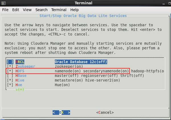
Description of this image Notes:
- If the service is started, close the terminal window, and move on to Step 3.
- If the service is not started, perform steps 2.A. through 2.C:
A. Use the down arrow key to highlight the HDFS option.
B. Press the Spacebar to select the option.
C. Press the Enter key to start the HDFS service. Note: After HDFS starts up, the terminal window automatically closes.
-
Enable proxy access in the browser. To do this:
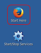
- Open the browser by using the Start Here desktop icon, as shown below.
- In the browser, right-click just above the Address box and enable the Menu Bar option.
- Then, select Edit > Preferences > Advanced > Network > Settings from the menu.
- In the Connection Settings dialog, select the Auto-detect proxy settings for this network option (as shown below) and click OK.
Description of this image 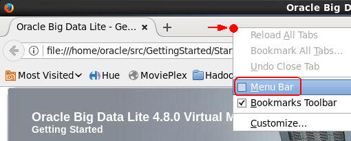
Description of this image 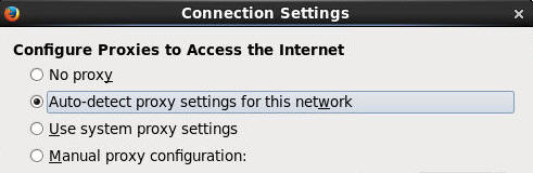
Description of this image -
Next, ensure that pop-up blocking is disabled. To do this:
A. select the Content category in the Preferences window navigator. In the Content window, deselect the Block pop-up windows option, as shown here:

Description of this image B. Close the browser.
-
Re-open the browser go to the Learn More section of the Big Data Spatial and Graph page at: http://www.oracle.com/technetwork/database/database-technologies/bigdata-spatialandgraph/learnmore/index.html. Then, perform the following:
A. Scroll down to the Hands On Lab section.
B. Click the "Applying Spatial Analysis to Big Data" link to download the BDL-4.6-Spatial-HOL.zip file. NOTE: Use the 'Save File' option in the menu.
- Close the browser and click the Terminal icon to open a terminal window, as shown here:

Description of this image NOTE: Hints for using code segments in the terminal window:
- To execute code, individually copy/paste code lines from the provided code segments to the command line interface.
- Then, execute each line of code at the command line by pressing
Enter. -
In the terminal window, execute the following lines of code to: A) Unzip the Vector-HOL.zip file to the specific directory, and B) Make the directory writeable.
cd Downloads unzip BDL-4.6-Spatial-HOL.zip cd BDL-4.6-Spatial-HOL/setup sudo unzip Vector-HOL.zip -d /opt/oracle/oracle-spatial-graph/spatial/vector/HOL sudo chmod -R 777 /opt/oracle/oracle-spatial-graph/spatial/vector/HOL -
Now, execute the following line of code to unzip the Raster-HOL.zip file to the specific directory.
sudo unzip Raster-HOL.zip -d /opt/oracle/oracle-spatial-graph/spatial/raster/ -
Finally, execute the following two lines of code to start Tomcat:
sudo service bdsg start
sudo service bdsg status
RESULT: The following output should appear: "Oracle BigData Spatial and Graph Consoles are started". This output, following the status command, indicates that the Tomcat servlet is running and Spatial consoles are started:
-
Next, create a working directory in HDFS by executing the following command:
hadoop fs -mkdir /user/oracle/HOL -
Finally, load the data for this tutorial into HDFS by executing the following four lines of code:
hadoop fs -put /opt/oracle/oracle-spatial-graph/spatial/vector/HOL/data/tweets.json /user/oracle/HOL/tweets.json
hadoop fs -put /opt/oracle/oracle-spatial-graph/spatial/vector/HOL/data/USA_2012Q4_PCB3_PLY.dbf /user/oracle/HOL/USA_2012Q4_PCB3_PLY.dbf
hadoop fs -put /opt/oracle/oracle-spatial-graph/spatial/vector/HOL/data/USA_2012Q4_PCB3_PLY.shp /user/oracle/HOL/USA_2012Q4_PCB3_PLY.shp
hadoop fs -put /opt/oracle/oracle-spatial-graph/spatial/vector/HOL/data/USA_2012Q4_PCB3_PLY.shx /user/oracle/HOL/USA_2012Q4_PCB3_PLY.shx
Use the Spatial Vector Console
In this section, the file /user/oracle/HOL/tweets.json will be used. This GeoJSON file contains sample tweets, which include geometry information, a location text, the number of followers, and the number of friends of the person who sent the tweet.
The API provides InputFormats and RecordInfoProvider implementation for the common formats GeoJSON and ESRI Shapefiles. It is possible to use any Hadoop provided or customized InputFormat and any customized RecordInfoProvider.
NOTE: For simplicity, these examples don’t use the MVSuggest data enrichment service and don’t send notification emails after job completions.
Create a Spatial Index
In this topic, you create an index on the file /user/oracle/HOL/tweets.json.
Follow these steps:
-
Launch the browser, and select Spatial and Graph > Oracle Spatial Vector Console from the toolbar, as shown here:
Description of this image - In the Spatial Hadoop Vector Console, click the Spatial Index tab, and then specify the following values:
- Index name: tweetsJanuaryIndex
- Path of data to the index: hdfs://bigdatalite.localdomain:8020/user/oracle/HOL/tweets.json
- New index path: hdfs://bigdatalite.localdomain:8020/user/oracle/HOL/tweetsIndex1
- SRID (of the geometries used to build the index): 8307
- Tolerance (to accommodate rounding errors): 0.5
- Input Format class (used to read the input data): oracle.spatial.hadoop.vector.geojson.mapred.GeoJsonInputFormat
- Record Info Provider class (provides spatial information): oracle.spatial.hadoop.vector.geojson.GeoJsonRecordInfoProvider
The completed New Index form should look like this:
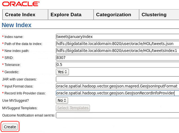
Description of this image -
As shown in the image above, click Create.
-
When the job is submitted, open a new Firefox tab and then go to http://localhost:8088/cluster/apps.
-
Close the Hadoop - FINISHED Applications tab.
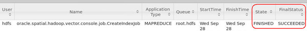
In the Hadoop - All Applications tab, click the FINISHED link, as shown here:
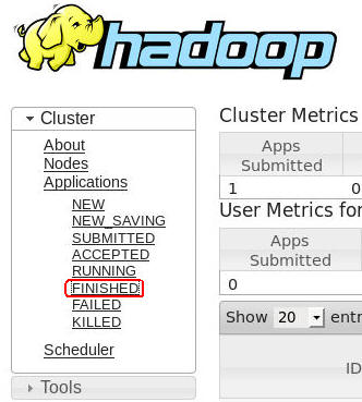
Note: When the job completes successfully, the log should show a State of FINISHED, and a FinalStatus of SUCCEEDED, as shown below.
Run a Categorization Job
Using the spatial index that you completed in the previous topic, you categorize the tweets in the file /user/oracle/HOL/tweets.json by Countries, States, and Provinces in order to determin how many tweets have been sent by country and by State or Province.
- In the Spatial Hadoop Vector Console, Select Categorization > Run Job.
- In the New Job form, select tweetsJanuaryIndex from the Index option, as shown below:

Description of this image -
Next, click the Select Templates button, and choose World Countries as hierarchy 1, and World State Provinces as hierarchy 2. Then click Save, as shown below:

Description of this image - Finally, complete the New Job form, as shown below:
- Output path: hdfs://bigdatalite.localdomain:8020/user/oracle/HOL/catOutput
- Name: Tweets January
- Click Create
-
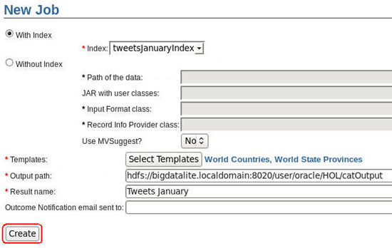
Description of this image -
Again, open http://localhost:8088/cluster/apps in a new Firefox tab. When the job is completes, you should see the Hierarchical job having finished successfully, as shown here:

Description of this image -
Toggle back to the Spatial Hadoop Vector Console tab and select Categorization > View Results.
-
First, in the Templates list, click on the World Countries. A Results category appears below the Templates list.
-
Then, click on Tweets January result. A color-coded map of the world countries appears. Note: You can zoom on the map by double-clicking the image.
Move the cursor over the United States to view the number of tweets in the US.
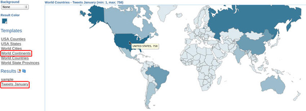
Description of this image -
Now, click the country United States.
Mouse over any state to view the number of tweets per state. In this example, the tweet count for Alaska is shown:
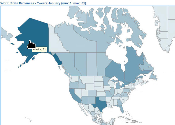
Description of this image NOTES: You can refersh the map and view other locations by selecting Templates > World Countries and Results > Tweets January on the left. When you are done viewing tweet results in the map, move on to the next exercise.
Run a Binning Job
In this topic, you run a binning analysis job on the tweets, using the same index that you created previously.
Follow these steps:
-
In the Spatial Hadoop Vector Console tab, select Binning-> Run Job.
-
Then, in the New Job form, select the With Index option and tweetsJanuaryIndex
- Change the binning grid minimum bounding rectangle (MBR) to the following values:
- Min. X = -175
- Max. X = 175
- Min. Y = -75
- Max. Y = 75
-
Then, click the Display MBR button (as shown below):
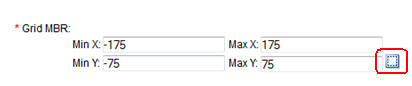
Description of this image Result: The following map appears in a new window.:
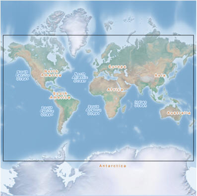
Description of this image -
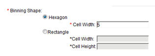
Back in the New Job form, set the Binning Shape to Hexagon, and the cell width of each hexagon is set to 5.
Description of this image -
Finally, use the following values for these remaining options:
- Leave the Thematic attribute option value as count. This value means that each cell in the grid will display the number of tweets associated with that cell.
- Output path: hdfs://bigdatalite.localdomain:8020/user/oracle/HOL/binningOutput
- Result Name: Tweets January
The completed New Job form should look like this:

Description of this image -
Now, click Preview to display a preview of the grid with empty hexagonal bins in the map window, as shown below:

Description of this image -
Finally, close the preview map and click Create in the New Job form.
NOTE: While the binning job is running, toggle back to the Applications tab in the browser to view the job log. Click the FINISHED link to refresh the log. Wait until log shows that the job completed successfully.
-
When the binning job is finshed, toggle back to the Spatial Hadoop Vector Console tab and select Binning > View Results to display the binning map.
-
In the options bar to the left of the map, select World Map as the Backround option, and click the Tweets January link under the Results heading.
Result: You may view the number of tweets in any cell moving the mouse cursor on it. As before, you can double-click on the map to zoom in.

Description of this image NOTES: The darker the color, the larger the number of tweets in that bin. When you are done viewing tweet results in the map, move on to the next exercise.
Run a Clustering Job
In this topic, you run a clustering analysis job on the tweets. The K–means clustering method is used and the number of clusters is 2.
NOTE: K-means is a popular method for clustering analysis in data mining. For more information, see: https://en.wikipedia.org/wiki/K-means_clustering.
Follow these steps:
- In the Spatial Viewer tab, select Clustering > Run Job.
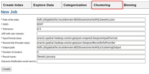
- Then, in the New Job form, specify the following values:
- Path of data: hdfs://bigdatalite.localdomain:8020/user/oracle/HOL/tweets.json
- SRID: 8307
- Tolerance: 0.5
- Input Format class: oracle.spatial.hadoop.vector.geojson.mapred.GeoJsonInputFormat
- Record Info Provider class: oracle.spatial.hadoop.vector.geojson.GeoJsonRecordInfoProvider
- Output path: hdfs://bigdatalite.localdomain:8020/user/oracle/HOL/clusteringOutput
- Number of clusters: 2
- Result Name: Tweets January
-
Click Create.
-
While the clustering job is running, toggle back to the Applications tab in the browser to view the job log. Click the FINISHED link to refresh the log. Wait until the log shows that the job has completed successfully.
-
When the job is finshed, toggle back to the console tab and select Clustering > View Results to display the clustering map.
-
In the options bar to the left of the map, select World Map as the Background and click the Tweets January link under the Results heading. Then, enable the Show clusters boundaries option.
Notes: The Tweets January cluster result may take a moment to appear in the viewer. Click the refresh tool (
 ) next to the Results heading until the list is updated.
Result: The map shows clusters centers and boundaries. As before, double click the image to zoom in.

Description of this image -
Mouse over a cluster to display the number of tweets inside that cluster. In this example, the East cluster has 2534 members, and the West cluster has 4169 members. Note: Your values may be slightly different.
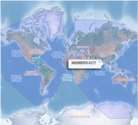
Description of this image -
When you are done, close the browser.
The New Job form should look like this:
Use the Command Line for Spatial Vector Analysis
In the previous section, you learned how to run jobs and display their results in the spatial vector console. Now, you learn how to run a spatial vector job from the command line.
In this section, you leverage of the libjars option in the hadoop jar command to make several required JAR’s available to mapReduce tasks. This is accomplished by creating an environment variable named HADOOP_LIB_JARS. This environment variable will reference the required jars.
Therefore, before you begin the exercises in this section, perform the following:
1. First, open a terminal window and execute the two export commands shown below.
export API_LIB_DIR=/opt/oracle/oracle-spatial-graph/spatial/vector/jlib
export HADOOP_LIB_JARS=$API_LIB_DIR/sdohadoop-vector.jar,$API_LIB_DIR/sdoapi.jar,$API_LIB_DIR/sdoutl.jar,$API_LIB_DIR/ojdbc8.jar,$API_LIB_DIR/hadoop-spatial-commons.jar
2. Then, to make these same JAR’s available to the client JVM, run the following command, which sets the HADOOP_CLASSPATH environment variable containing the needed jars.
export HADOOP_CLASSPATH=$API_LIB_DIR/sdohadoop-vector.jar:$API_LIB_DIR/sdoapi.jar:$API_LIB_DIR/sdoutl.jar:$API_LIB_DIR/ojdbc8.jar:$API_LIB_DIR/hadoop-spatial-commons.jar:$HADOOP_CLASSPATHCreate a Spatial Index Using a GeoJSON File
In this topic, you create a spatial index using a job named oracle.spatial.hadoop.vector.mapred.job.SpatialIndexing.
This job requires a variety of agruments to define the parameters for the index creation process. The parameters are similar to those that you used in the Vector Console form, when creating the vector index for the previous exercise.
The job:
- Uses the file /user/oracle/HOL/tweets.json as input data for the index
- Creates an index named indexGeoJSON
- Generates metadata for the index in a specified directory
To generate the index, follow these steps:
-
Using the terminal window, execute the following long line of code to generate the index:
hadoop jar $API_LIB_DIR/sdohadoop-vector.jar oracle.spatial.hadoop.vector.mapred.job.SpatialIndexing -libjars $HADOOP_LIB_JARS input=/user/oracle/HOL/tweets.json output=/user/oracle/HOL/indexGeoJSON inputFormat=oracle.spatial.hadoop.vector.geojson.mapred.GeoJsonInputFormat recordInfoProvider=oracle.spatial.hadoop.vector.geojson.GeoJsonRecordInfoProvider srid=8307 geodetic=true tolerance=0.5 indexName=indexGeoJSON indexMetadataDir=/user/oracle/indexMetadata overwriteIndexMetadata=trueOnce the job is finished, the message "INFO: Job Succeeded" appears in the output.
Run a Categorization Job Using a Custom Layer
In this topic, you run a job that categorizes tweets by countries and regions inside the eurozone.
Since the API doesn’t provide the needed country and region data sets, the job will use two JSON format files: eurozone_countries.json and eurozone_provinces.json.
In addition, a HierarchyInfo class is called by the job. This class describes the hierarchies that are used to categorize the tweets data. The first hierarchy is the eurozone_countries and the second hierarchy is the eurozone_provinces.
An image of the class implementation is shown here:
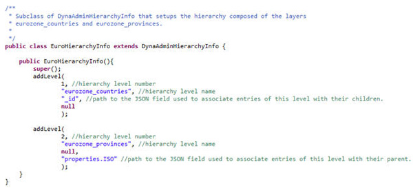
Note: The class is contained in a jar file named eurohierarchyinfo.jar.
Follow these steps:
-
Using the open terminal window, execute the following two export commands to make eurohierarchyinfo.jar available for Hadoop:
export HADOOP_CLASSPATH=/opt/oracle/oracle-spatial-graph/spatial/vector/HOL/jlib/eurohierarchyinfo.jar:$HADOOP_CLASSPATH export HADOOP_LIB_JARS=/opt/oracle/oracle-spatial-graph/spatial/vector/HOL/jlib/eurohierarchyinfo.jar,$HADOOP_LIB_JARS -
Now run the categorization job by executing the following command in the terminal window:
hadoop jar $API_LIB_DIR/sdohadoop-vector.jar oracle.spatial.hadoop.vector.mapred.job.Categorization -libjars $HADOOP_LIB_JARS spatialOperation=IsInside input=/user/oracle/HOL/tweets.json output=/user/oracle/HOL/euroZoneCatOutput inputFormat=oracle.spatial.hadoop.vector.geojson.mapred.GeoJsonInputFormat recordInfoProvider=oracle.spatial.hadoop.vector.geojson.GeoJsonRecordInfoProvider srid=8307 geodetic=true tolerance=0.5 hierarchyInfo=hol.EuroHierarchyInfo hierarchyIndex=/user/oracle/HOL/hierarchyIndex hierarchyDataPaths=file:///opt/oracle/oracle-spatial-graph/spatial/vector/HOL/data/eurozone_countries.json,file:///opt/oracle/oracle-spatial-graph/spatial/vector/HOL/data/eurozone_provinces.jsonNote: Once the job completes, the message "INFO: Job Succeeded" appears in the output. In addition, the result is saved in the HDFS folder /user/oracle/HOL/euroZoneCatOutput.
-
Using the terminal window, execute the following command to copy the output locally:
sudo hadoop fs -get /user/oracle/HOL/euroZoneCatOutput/*.json -
Then, execute the ls command to view a listing of the tweet count output files:
ls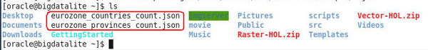
Description of this image -
Execute the following command to view some of the data for the eurozone contries count output:
more eurozone_countries_count.jsonA portion of the count output is shown here:

Description of this image Notes:
Each record id refers to the record in the eurozone_countries.json file. For example:
- The count result highlighted in the image above ({"id":"FRA","result":62}) refers to the following record in the file eurozone_countries.json:
- {"type":"Feature","_id":"FRA","geometry":{"type":"Polygon","coordinates":[[1.44136,42.60366,1.47851,42.65168,…,1.44136,42.60366]]},"properties":{"Continent":"EU","Name":"France","Alt_Region":"EMEA","Country Code":"FRA"},"label_box":[-1.12061,45.13915,6.02255,49.19591]}
-
Close any open terminal windows.
In this case, we see that 62 tweets have been sent from France.
Want to Learn More?
-
For more practice on job customization, see additional code examples on the Big Data Lite VM at: /opt/oracle/oracle-spatial-graph/spatial/vector/examples.
-
For customized job examples, see additional exercises at: http://www.oracle.com/technetwork/database/database-technologies/bigdata-spatialandgraph/learnmore/index.html -> Hands On Labs -> Applying Spatial Analysis to Big Data/opt/oracle/oracle-spatial-graph/spatial/vector/examples.